Segment nuclei with StarDist
This example opens a 3D microscopy image from an icechunk repository on Arraylake and segments its nuclei in Fiji with StarDist, a deep learning model that runs in Python.
- The example opens the image by URL, takes 20 slices of its nuclear stain, and runs StarDist on them.
- The image is
idr0062Afrom Earthmover's demo copy of the Image Data Resource (IDR). It comes from idr0062, a study of nuclear segmentation in mouse tissue imaged by confocal microscopy: two channels, LaminB1 and DAPI, 271 × 275 pixels and 236 slices. - Appose runs the Python. It builds a Python environment from the packages a
script names, runs the script in a separate worker process, and passes images through shared memory instead of
copying them. A Script Editor script that starts with
#@script (language="appose-python")runs this way, so nothing is installed by hand beyond the Fiji setup. The Appose workshop covers writing such scripts.
What you need
- Fiji set up as in Use in Fiji, with the icechunk-arraylake-java jar added, since the image is on Arraylake.
- An Arraylake login. The repository is readable by any signed-in Arraylake user. The jar uses the login that the
Python client writes, so run
arraylake auth loginonce with the Arraylake Python client. - Appose Python scripting, which ships with Fiji on the Fiji-Latest update site. The Script Editor lists it under Templates > Appose.
Open the image
- Choose File > Import > HDF5/N5/Zarr/OME-NGFF ....
-
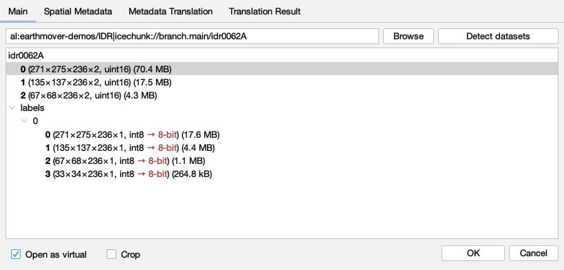
Paste this URL into the dataset field:
al:earthmover-demos/IDR|icechunk://branch.main/idr0062A -
Click Detect datasets. The tree lists three resolution levels,
0to2, and alabelsgroup. - Select
0, the full-resolution array, tick Open as virtual, and click OK.
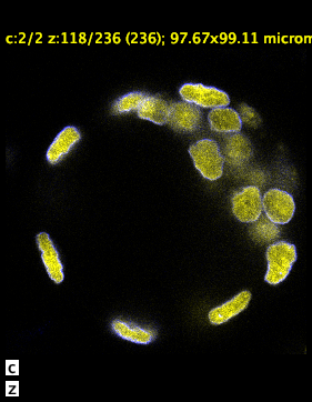
The image opens as a 2-channel stack of 236 slices. With Open as virtual, Fiji reads a slice from Arraylake only when it is shown, so the window appears in a few seconds. The data is dim against the full 16-bit range and can look black at first: choose Process > Enhance Contrast with the default 0.35% saturated pixels.
Take the DAPI slices
StarDist's fluorescence model expects one nuclear-stain channel, and the script segments one slice at a time. Choose Image > Duplicate... and set:
| Field | Value |
|---|---|
| Title | idr0062A DAPI |
| Channels (c) | 2 |
| Slices (z) | 110-129 |
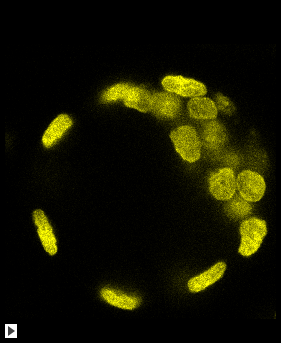
Fiji reads those 20 slices of the DAPI channel from Arraylake and opens them as an ordinary in-memory stack. Close the virtual image if you no longer need it, and run Process > Enhance Contrast on the new stack.
Run StarDist
- Open the Script Editor (File > New > Script...) and choose Templates > Appose > StarDist cellcast.
-
With the
idr0062A DAPIwindow active, click Run. The script takes the active image as its input and asks for its parameters. The defaults suit this image.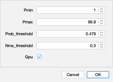
-
Click OK.
The first run downloads and installs a Python environment with cellcast, which
provides StarDist, before it segments anything. Later runs reuse the environment and finish the 20 slices in a few
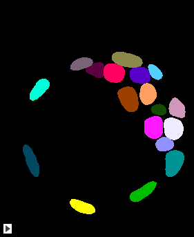
seconds. The result opens as a labels stack of the same size, with each nucleus a different integer. To colour the
labels, choose Image > Lookup Tables > glasbey on dark.
The template is
StarDist_cellcast.py
from scripting-appose-python. Its header names the Python
packages it needs, and Appose builds the environment from that header.
To keep the labels, and each later run's labels alongside them, save them into an icechunk repository: Example: save results into icechunk shows how.